Linear Transformations
Lecture 5
Recap
$$ % Colors
% Coordinate vectors and matrices
% Common sets
% Abstract vector symbols
% Norms / absolute value
% Optional: dot product spacing (looks nicer in slides)
% Operators $$
Coordinate system
- Let an \(n \times k\) matrix \(A = [\vec{v}_1 \ \cdots \ \vec{v}_k]\) consist of \(k\) column vectors in \(\mathbb{R}^n\).
- Each vector \(\vec{v}_j\) can be interpreted as an axis direction of a new coordinate system, expressed in the Cartesian coordinate system.
- Let a \(k \times m\) matrix \(C = [\vec{c}_1 \ \cdots \ \vec{c}_m]\) consist of the coordinates (in the \(A\)-system) of \(m\) points as its column vectors.
- The matrix multiplication \(AC = W = [\vec{w}_1 \ \cdots \ \vec{w}_m]\) produces column vectors representing the same points, now written in the Cartesian coordinate system.
Exercise
- Consider a coordinate system with axis directions \(\vec{v}_1 = \langle 1,-1 \rangle\) and \(\vec{v}_2 = \langle 0,2 \rangle\).
- Draw a grid generated by these two vectors. Note that each cell is no longer a square.
- Plot the point with coordinates \((2,1)\), interpreted as “move the origin by 2 units in the \(\vec{v}_1\) direction and 1 unit in the \(\vec{v}_2\) direction.”
- Find the Cartesian coordinates of that point from your picture.
- Verify your answer using a matrix multiplication \[[\vec{v}_1 \quad \vec{v}_2]\begin{bmatrix} 2 \\ 1 \end{bmatrix}.\]
Linear Transformations
New interpretation
- The matrix \(A\) describing the axes is fixed, and we can multiply any coordinate vector \(\vec{c} \in \mathbb{R}^k\) by \(A\) to obtain a vector \(\vec{w} \in \mathbb{R}^n\), that is, \(A\vec{c} = \vec{w}\).
- Keep track of dimensions: the axes live in \(\mathbb{R}^n\), we combine \(k\) of them using a coordinate vector in \(\mathbb{R}^k\), and the result lies in \(\mathbb{R}^n\).
- This can be interpreted as \(A\) transforms \(\vec{c}\) into \(\vec{w}\).
Matrix multiplication as function
- Let \(\vec{x} = \begin{bmatrix} x_1 \\ \vdots \\ x_k \end{bmatrix}\) be a point in \(\mathbb{R}^k\).
- Then \(A\vec{x} = \vec{y} = \begin{bmatrix} y_1 \\ \vdots \\ y_n \end{bmatrix}\) is a point in \(\mathbb{R}^n\).
- We write \(\vec{y} = A(\vec{x}) = A\vec{x}\) and interpret \(A:\mathbb{R}^k\to \mathbb{R}^n\) as a function.
- A function represented by multiplication by a matrix is called a linear transformation.
- Geometrically, a point in \(\mathbb{R}^k\) is transformed linearlly into a point in \(\mathbb{R}^n\).
Linear transformations
- A vector \(\vec{x} = \langle x_1, \dots, x_k \rangle = x_1 \vec{e}_1 + \dots + x_k \vec{e}_k\) represents a point in \(\mathbb{R}^k\) with respect to the Cartesian coordinate system.
- Instead of the standard basis \(\vec{e}_1, \dots, \vec{e}_k\), we choose vectors \(\vec{v}_1, \dots, \vec{v}_k \in \mathbb{R}^n\) as new axes.
- Using the same coordinates \((x_1,\dots,x_k)\), we obtain \[ \vec{y} = x_1 \vec{v}_1 + \dots + x_k \vec{v}_k \in \mathbb{R}^n. \]
Note: In the previous class, matrix multiplication was used to convert coordinates between different coordinate systems. Here, the coordinate system is fixed, and matrix multiplication maps one point to another point.
Visualizing linear transformations
\(A:\mathbb{R}\to\mathbb{R},\quad n = k = 1\)
- When \(n = k = 1\), a matrix reduces to a single number \([a]\), and the linear transformation is \(y = ax\).
- The coordinate vector \(\langle 1 \rangle\) in \(\mathbb{R}\) is replaced by \(\langle a \rangle\) in \(\mathbb{R}\) with this transformation, so a point \(x = x\cdot 1\) is mapped to \(y = x\cdot a\).
- Thus, the \(1\times 1\) matrix \([a]\) represents scaling of the real line by a factor of \(a\).
\(A:\mathbb{R}\to\mathbb{R}^2,\quad n = 2, k = 1\)
- Let \(A = [\vec{v}] = \begin{bmatrix} v_1 \\ v_2 \end{bmatrix} \in \mathbb{R}^2\). The associated transformation is \(\vec{y} = A x\) for \(x \in \mathbb{R}\).
- The coordinate vector \(\langle 1 \rangle\) in \(\mathbb{R}\) is replaced by \(\vec{v}\) in \(\mathbb{R}^2\), so \(\vec{y} = x\cdot \vec{v} = \langle x v_1, x v_2 \rangle\) (from \(x=x\cdot 1\)).
- Geometrically, \(\vec{y}\) lies on the line obtained by expanding \(\vec{v}\).
\(A:\mathbb{R}^2\to\mathbb{R},\quad n = 1,\; k = 2\)
- Let \(A = [\,a \quad b\,]\) be a \(1\times 2\) matrix. Although it has two entries, \(A\) represents two coordinate vectors \(\langle a \rangle, \langle b \rangle\in\mathbb{R}\)—it does not represent a single vector in \(\mathbb{R}^2\).
- The vector \(\vec{x}=\begin{bmatrix}x_1\\ x_2\end{bmatrix} = x_1\vec{e}_1 + x_2\vec{e}_2 \in \mathbb{R}^2\) is transformed into \[\vec{y}=A\vec{x}=ax_1+bx_2.\]
- The basis vectors \(\vec{e}_1\) and \(\vec{e}_2\) are replaced by \(\langle a \rangle\) and \(\langle b \rangle\) in \(\mathbb{R}\).
Note: This transformation maps a vector to a scalar. We will later revisit this idea in the context of the scalar product (also called the dot product or inner product).
\(A:\mathbb{R}^2\to\mathbb{R}^2,\quad n = k = 2\)
- When \(n = k = 2\), a \(2\times 2\) matrix maps points in the plane to other points in the plane.
- Writing \(A = [\,\vec{v}_1 \ \vec{v}_2\,]\), the columns give the images of the basis vectors \(\vec{e}_1\) and \(\vec{e}_2\), and thus define new axis directions.
- Explicitly, for \(\vec{x}=\langle x_1,x_2 \rangle=x_1\vec{e}_1+x_2\vec{e}_2\), we have \[\vec{y}=A\vec{x}=x_1\vec{v}_1+x_2\vec{v}_2.\]
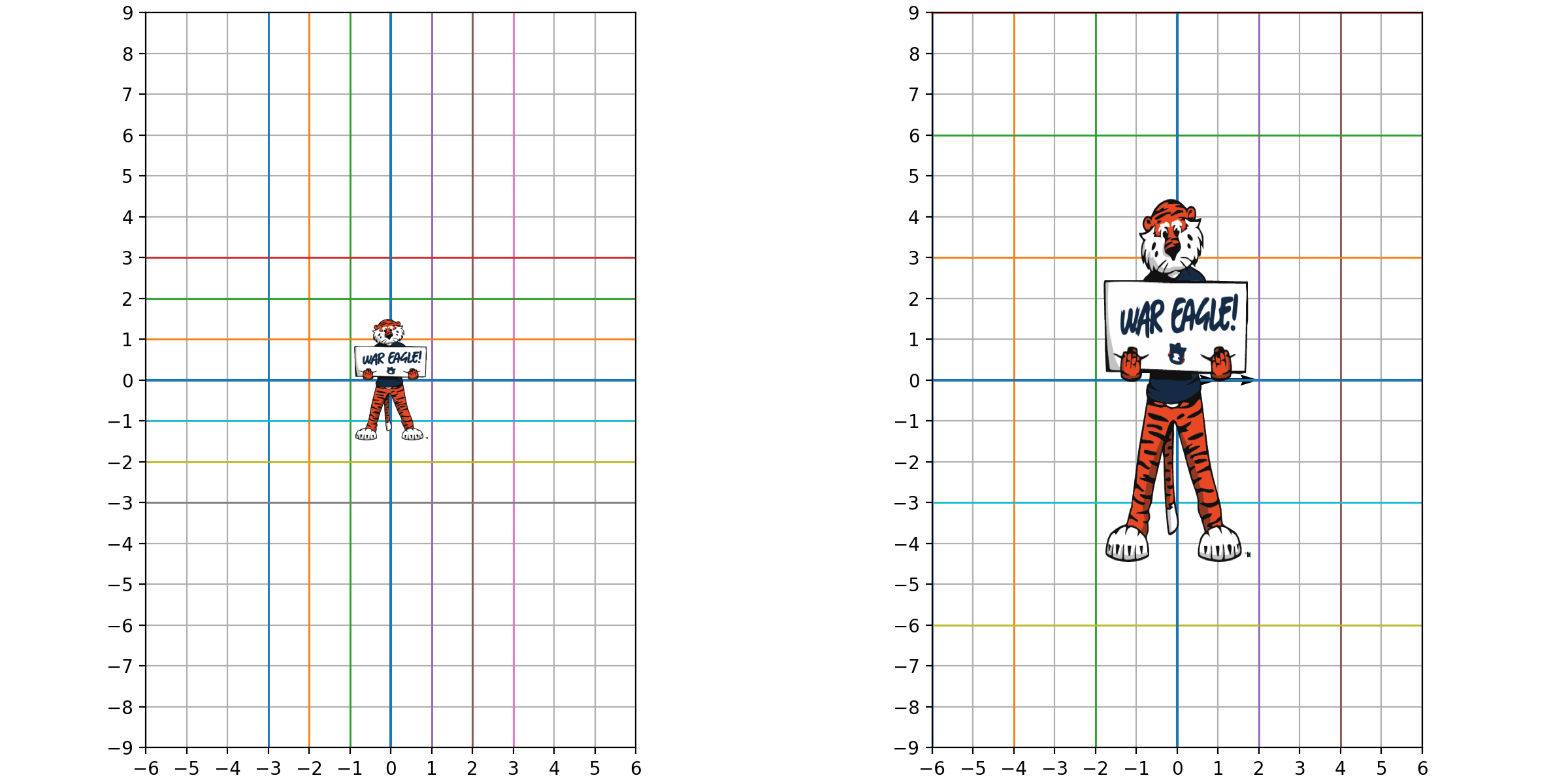
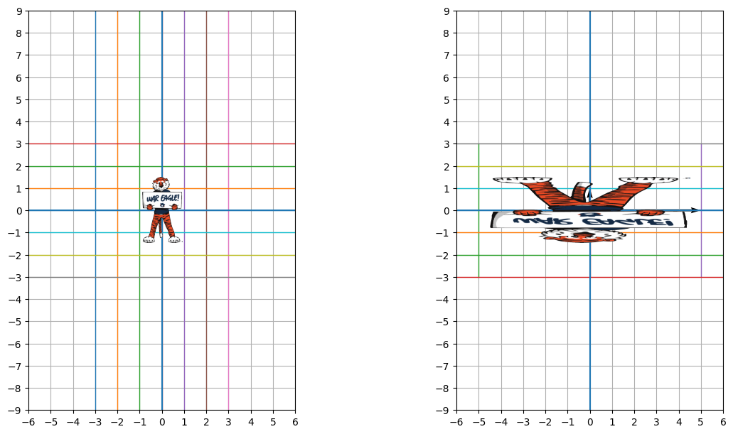
Example 1: \(2\times 2\) diagonal matrices
- A diagonal matrix has the form \(A = \begin{bmatrix} a & 0 \\ 0 & b \end{bmatrix}\).
- Then \(A \begin{bmatrix} x_1 \\ x_2 \end{bmatrix} = \begin{bmatrix} a x_1 \\ b x_2 \end{bmatrix}\).
- Note that coordinate vectors \(\vec{e}_1 = \langle 1,0 \rangle\) and \(\vec{e}_2=\langle 0,1 \rangle\) are replaced by \(\langle a,0 \rangle=a\vec{e}_1\) and \(\langle 0, b \rangle=b\vec{e}_2\).
- Each coordinate direction is scaled independently.
\(A(x, y) = (2x, 3y)\)
\(A(x, y) = (5x, -y)\)
Example 2: \(2\times 2\) transpose matrices
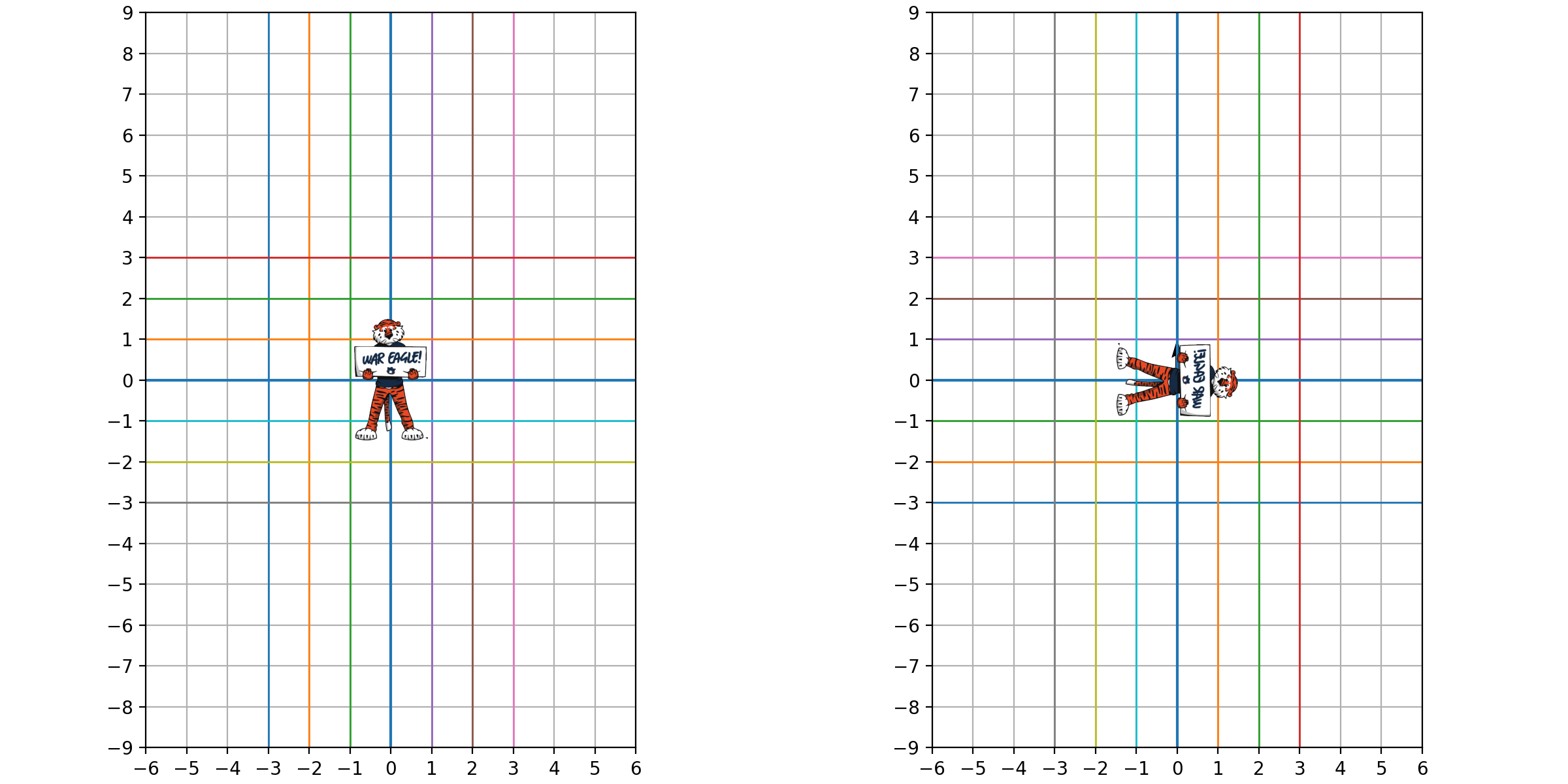
- Consider \(A = \begin{bmatrix} 0 & 1 \\ 1 & 0 \end{bmatrix}\).
- Then \(A \begin{bmatrix} x_1 \\ x_2 \end{bmatrix} = \begin{bmatrix} x_2 \\ x_1 \end{bmatrix}\).
- Under this transformation, \(\vec{e}_2\) plays the role of the first coordinate vector, and vice versa.
- This matrix swaps the two coordinates, so it is called a transpose matrix.
\(A(x, y) = (y, x)\)
Example 3: \(2\times 2\) rotation matrices
- The rotation matrix is \(A = \begin{bmatrix} \cos \theta & -\sin \theta \\ \sin \theta & \cos \theta \end{bmatrix}\).
- Geometrically, it rotates each unit coordinate vector \(\vec{e}_i\) by angle \(\theta\).
- As a result, every point in the plane is rotated by angle \(\theta\) about the origin.
Rotation by \(30^\circ\)

Observation
- A linear transformation \(A\) can be understood by how it acts on the coordinate vectors \(\vec{e}_i\).
- For example, if \(\vec{e}_1\) is mapped to \(3\vec{e}_1\), then the transformation stretches the \(x\)-direction by a factor of \(3\).
- In general, if \(A\vec{e}_i=\vec{v}_i\), then the matrix representation of \(A\) is \[A=[\vec{v}_1\ \cdots\ \vec{v}_k].\]
Example 4: \(2\times 2\) shear matrices
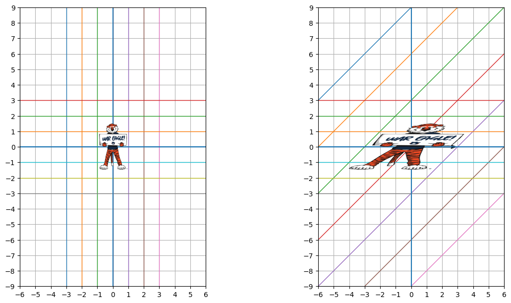
- Consider the matrix \[A=\begin{bmatrix}1&1\\0&1\end{bmatrix}.\]
- The image of the first coordinate vector is \(\vec{e}_1=\langle 1,0 \rangle\), so there is no change in the \(x\)-direction.
- The image of the second coordinate vector is \(\langle 1,1 \rangle\), which means the \(y\)-direction is sheared in the \(x\)-direction.
\(A(x,y)= (3x+y, y)\)
Summary
- A linear transformation \(A:\mathbb{R}^k \to \mathbb{R}^n\) maps a vector \(\vec{x}\in\mathbb{R}^k\) to \(A\vec{x}\in\mathbb{R}^n\) via multiplication by an \(n\times k\) matrix \(A\).
- The transformation is completely determined by its action on the coordinate vectors \(\vec{e}_i\in\mathbb{R}^k\), sending each to a vector \(\vec{v}_i\in\mathbb{R}^n\).
- Each vector \(\vec{v}_i=A(\vec{e}_i)\) appears as the \(i\)-th column of \(A\). Equivalently, knowing \(A(\vec{e}_i)\) for all \(i\) determines the matrix.
- In low dimensions—especially in the plane—these effects can often be visualized geometrically.